1 / 1

Releasing the Pressure

High-order surface flow discretizations via
discrete Helmholtz–Hodge decompositions

Tim Brüers · Christoph Lehrenfeld · Tim van Beeck · Max Wardetzky
Institute for Numerical and Applied Mathematics · University of Göttingen
NGSolve User Meeting · 2026
QR code linking to these slides

MotivationIncompressible flows on curved surfaces

  • Arise in thin-film dynamics, biomembranes, and geophysical flows
  • Two geometric constraints on the velocity $\uu$:
    • tangential to the surface
    • divergence-free
  • $\Hdiv$-conforming BDM elements satisfy both exactly:
    • pointwise divergence-free
    • tangential
    • pressure-robust
  • need to solve velocity–pressure saddle-point system.
A von Kármán vortex street on the NGSolve sculpture.

SettingThe surface (Navier–)Stokes equations

On a surface $M\subset\mathbb{R}^3$ find a tangential velocity $\uu$ and pressure $p$:

Surface Stokes
$$ \begin{aligned} -\mu\,\dive(\strain(\uu)) + \grad p &= \ff \\ \dive\uu &= 0 \end{aligned} $$
Unsteady surface Navier–Stokes  ($\mu=0$: Euler)
$$ \begin{aligned} \partial_t\uu + \partial_{\uu}\uu - \mu\,\dive(\strain(\uu)) + \grad p &= \ff \\ \dive\uu &= 0 \end{aligned} $$
Triangulated surface mesh of a torus
model surface $M$

Operators on the surface

With $J$ the rotation by $90^\circ$:

$$ \rot := -J\,\grad,\qquad \curl := -\dive J $$
The key idea

Skip the saddle point —
work directly in the divergence-free subspace

Solve directly inside $\JL=\{\,\uu\in\mathbf{H}(\dive) : \dive\uu=0\,\}$, which splits as

$$ \JL \;=\; \rot(\textcolor{#6c8cff}{\text{streamfunction}}) \;\oplus_{L^2}\; \textcolor{#ff7d6b}{\text{harmonic part}} $$
no pressure no saddle point exact tangentiality pointwise div-free pressure-robust high order

ObservationTopology matters

Divergence-free field on a simply connected bunny
Divergence-free field on a bunny with a handle

Theory · smooth surfaceThe Helmholtz–Hodge decomposition

$$ \mathbf{H}^1(M) = \grad\big(H^2\!\cap H^1_0\big)\ \oplus_{L^2}\ \rot\big(H^2\!\cap H^1_0\big)\ \oplus_{L^2}\ \mathbf{H}_N(M) $$

An $L^2$-orthogonal split into a gradient, a streamfunction rotation, and a harmonic field.

Total divergence-free field \(=\) Gradient component \(\oplus\) Streamfunction rotation component \(\oplus\) Harmonic component total field gradient streamfunction rotation harmonic

Why it mattersTopology lives in the harmonic part

  • For a divergence-free field the gradient term drops:
    $$ \mathbf{H}^1\!\cap\JL = \rot(H^2\!\cap H^1_0)\ \oplus_{L^2}\ \mathbf{H}_N(M) $$
  • The harmonic space $\mathbf{H}_N(M)$ is finite-dimensional:
    $$ \dim \mathbf{H}_N(M) = b_1(M) \quad(\text{first Betti number}) $$
  • It captures circulation around non-contractible loops, i.e., the net flow a streamfunction can never describe.
Harmonic field on a torus
The harmonic field on a torus — circulation around a non-contractible loop.

From smooth to discreteThe structure we want to keep

The smooth divergence-free space splits with the harmonic part capturing the topology:

$$ \mathbf{H}^1\!\cap\JL = \rot(H^2\!\cap H^1_0)\ \oplus_{L^2}\ \mathbf{H}_N(M),\quad \dim\mathbf{H}_N = b_1(M) $$

Should be inherited by discrete velocity space:

$$ \Jbb_h = \rot(\Sbb_h)\ \oplus_{L^2}\ \Hbb_h,\qquad \dim\Hbb_h = b_1(M) $$

!Not for free

Naive discretization gets the harmonic dimension wrong — spurious modes appear or genuine ones vanish, and the topology is broken.

?The question

What property of the discrete spaces guarantees the right split?

The answer · FEECDiscretize the complex, not the equation

The split comes from the de Rham chain complex, and the harmonic fields(...) are precisely its cohomology.

$$ \begin{array}{ccccc} H^1_0 &\xrightarrow{\ \rot\ }& \mathbf{H}_0(\mathrm{div}) &\xrightarrow{\ \dive\ }& L^2_0 \\[2pt] \big\downarrow & & \big\downarrow & & \big\downarrow \\[2pt] \Sbb_0^{k+1} &\xrightarrow{\ \rot\ }& \BDM_0^{k} &\xrightarrow{\ \dive\ }& \mathbb{P}^{k-1} \end{array} $$

A finite-element sub-complex linked to the continuous one by commuting projections.

Cohomology is preserved

A compatible sub-complex reproduces the cohomology of the continuous complex — the central principle of FEEC.

#Topology is exact

The only non-trivial cohomology has dimension $b_1(M)$ — which forces the right harmonic count:

$$ \dim\big(\Hbb^k_\BDM\big) = b_1(M) $$
Main theoretical result

The discrete divergence-free space splits

Exactly the smooth decomposition — now realized in the BDM space:

$$ \Jbb^k_\BDM \;=\; \rot\big(\Sbb_0^{k+1}\big)\ \oplus_{L^2}\ \Hbb^k_\BDM $$

a direct dimension-counting argument — no FEEC machinery needed

Streamfunction

Continuous Lagrange $\Sbb_0^{k+1}$ — one scalar field $\psi_h$.

Harmonic

$\Hbb^k_\BDM$ — just $b_1(M)$ coefficients $\hh_h$.

Velocity

Recovered exactly: $\uu_h=\rot(\psi_h)+\hh_h$.

ConsequenceA pressure-robust, saddle-point-free problem

Find $\uu_h=\rot(\psi_h)+\hh_h\in\Jbb^k_\BDM=\rot(\Sbb_0^{k+1})\ \oplus_{L^2}\ \Hbb^k_\BDM$ such that

$$ \mathcal{F}_h\big(\rot(\psi_h)+\hh_h,\ \rot(\phi_h)+\mathbf{k}_h\big) = f_h\big(\rot(\phi_h)+\mathbf{k}_h\big) $$

Algorithm 4.1Randomized harmonic basis

$\Hbb^k_\BDM$ has no local basis. We build an $L^2$-orthonormal basis in $b_1(M)$ steps — succeeding with probability one.

Random divergence-free sample. Draw a random $\rr_h$ and project it into the divergence-free subspace via the Helmholtz projection $\Pi_{\Jbb^k_\BDM}$.

Remove the streamfunction part. Solve a Laplace problem for $\psi_h$ and subtract $\rot(\psi_h)$ — what remains is a candidate harmonic field.

Orthogonalize & accept. Gram–Schmidt against the current basis; if non-zero, normalize and keep. Repeat until $b_1(M)$ vectors are found.

From geometry to meshPiercing the bunny

Load .stp geometry
Cut hole + smoothing
Extract surface mesh
bunny.pyngsolve
from netgen.occ import OCCGeometry, Cylinder, Pnt, Y
import netgen.meshing as meshing

# load the CAD geometry of the bunny
occgeoshape = OCCGeometry("bunny.stp").shape
# pierce a cylindrical hole through the body
cyl   = Cylinder(Pnt(5, -300, 32), Y, r=10, h=500)
shape = occgeoshape - cyl

if smooth_hole:                       # round off the rim
    shape = shape.MakeFillet(shape.edges, 2)
shape  = shape.Scale(Pnt(0, 0, 0), 0.01)
occgeo = OCCGeometry(shape)

# mesh the surface only — a closed 2-manifold
ngmesh = occgeo.GenerateMesh(
    perfstepsend=meshing.MeshingStep.MESHSURFACE,
    maxh=maxh, minh=0.5*maxh, grading=0.7)

from ngsolve import Mesh
mesh = Mesh(ngmesh)
Loaded bunny geometry
Bunny with a pierced cylindrical hole
Bunny with the hole rim rounded off by fillets

In code · comparisonSaddle-point HDG vs. the streamfunction solver

stokes_hdg.pyvelocity–pressure
a  = BilinearForm(𝔹𝔻𝕄)
a += (gradu | gradv) * ds(...)
a += (gradu*n | tang(vhat-v.Trace())) \
        * ds(..., element_boundary=True)
a += (gradv*n | tang(uhat-u.Trace())) \
        * ds(..., element_boundary=True)
a += alpha*order**2/h \
        * (tang(vhat-v.Trace())
           | tang(uhat-u.Trace())) \
        * ds(..., element_boundary=True)

a += -div(u.Trace()) * q.Trace() * ds(...)
a += -div(v.Trace()) * p.Trace() * ds(...)
surface_stokes.pystreamfunction
a  = BilinearForm(ℙᵏ)
a += (gradu | gradv) * ds(...)
a += (gradu*n | tang(vhat-v.Trace())) \
        * ds(..., element_boundary=True)
a += (gradv*n | tang(uhat-u.Trace())) \
        * ds(..., element_boundary=True)
a += alpha*order**2/h \
        * (tang(vhat-v.Trace())
           | tang(uhat-u.Trace())) \
        * ds(..., element_boundary=True)

aemb = emb.T @ a.mat @ emb

Numerical experiments · validationEquivalent to velocity–pressure — at lower cost

Steady surface Brinkman problem on the torus, $k=2$. Relative $L^2$ discrepancy to the velocity–pressure HDG of [Lederer et al.]:

$N_{\mathcal T}$$\|\uu^{\mathrm{vp}}-\uu^{\mathrm{sf}}\|/\|\uu^{\mathrm{vp}}\|$$\|\dive\uu^{\mathrm{sf}}\|$
7823.6 × 10⁻⁸3.9 × 10⁻¹¹
12143.4 × 10⁻⁹8.8 × 10⁻¹¹
47402.8 × 10⁻⁸1.9 × 10⁻⁹

Discrete velocities agree up to solver / quadrature tolerances and stay divergence-free.

Fewer degrees of freedom

Trefoil knot, $k=2$, genus 1:

Streamfunction–harmonic
$27\,920 + 2$ total dofs
Velocity–pressure
$48\,860 + 20\,940 = 69\,800$ total dofs

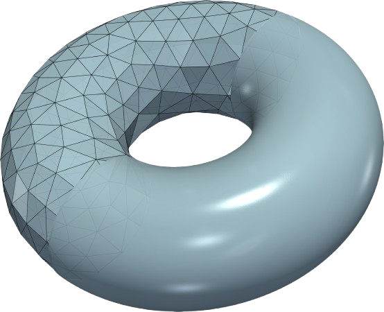
Experiment · genus 1Trefoil knot

  • A closed, orientable tube embedded as a knot: topologically a torus of genus $g=1$.
  • Number of harmonic fields is the first Betti number $b_1(M)=2g$.
  • Computable from the mesh via the Euler characteristic:
    $$ \chi(M)=V-E+F=2-2g \;\;\Longrightarrow\;\; b_1(M)=2-\chi(M) $$
Triangulated trefoil knot surface mesh
The trefoil knot surface $M$ has $b_1(M)=2$.

Experiment · genus 1The trefoil flow in motion

Transport circulates along the knot while cross-sectional vortices form around each tube section.

Experiment · genus 0, with boundaryPierced sculpture surface

  • Sphere with three large holes and one small hole (genus 0), four boundary rims, $\dim\Hbb^k_\BDM=3$.
  • Rigid-body-rotation forcing, no-slip rims, $k=4$; the small hole triggers a Kármán vortex street.
  • Again the harmonic part dominates the initial transient and the final quasi-periodic regime, concentrated on the smallest hole.
Triangulated pierced sculpture surface mesh
The pierced sculpture surface $M$ — genus 0 with four boundary rims, $\dim\Hbb^k_\BDM=3$.

Experiment · genus 0, with boundaryThe sculpture flow in motion

Vortex shedding off the small hole drives a Kármán street; the harmonic component carries the large-scale circulation.

In summaryReleasing the pressure

Discrete HH decomposition

The BDM divergence-free space splits exactly into a streamfunction rotation and a harmonic field.

Topology is captured

$\dim\Hbb^k_\BDM=b_1(M)$: the discrete complex preserves cohomology on surfaces of any topology

No saddle point

Solve with a scalar streamfunction + finitely many harmonic coefficients. Exact tangentiality, pointwise div-free, pressure-robust, high order.

Thank you

Questions welcome

Brüers · Lehrenfeld · van Beeck · Wardetzky — University of Göttingen

Code & data: GRO.data · 10.25625/VDG4OZ Animations: youtu.be/DqHXLNkhF0o
QR code linking to these slides

Implemented in Netgen/NGSolve with the NGSTrefftz add-on.

Overview — click a slide  ·  press Esc to close